python3とtensorflowによる最初の深層学習

次のコードでネットワークから実験用のデータを取得して、「iris_training.csv」のファイルに記憶します。

# -*- coding: utf-8 -*-
# <meta charset="utf-8"> iris_0.py
import os
import urllib.request
IRIS_TRAINING_CSV = 'iris_training.csv'
IRIS_TRAINING_URL = 'http://download.tensorflow.org/data/iris_training.csv'
if os.path.isfile( IRIS_TRAINING_CSV ) == True :
   print(IRIS_TRAINING_CSV,"のファイルが存在しているので、なにもしません。")
else:
   print(IRIS_TRAINING_URL,"から情報を取得して、ファイルを生成します。")   
   d = urllib.request.urlopen( IRIS_TRAINING_URL ).read();
   print(type(d)) # 
   s = d.decode()   # バイトを文字列へ変換 s = str(d) では正しく改行できなかった。
   for v in s.split( '\n' ):
       print(v)
   #
   with open( IRIS_TRAINING_CSV ,'wb' ) as f:
      f.write(d)
   #
   print("ネット情報から",IRIS_TRAINING_CSV,"のファイル生成しました。")   

この実行画面を示します。

http://download.tensorflow.org/data/iris_training.csv から情報を取得して、ファイルを生成します。

120,4,setosa,versicolor,virginica
6.4,2.8,5.6,2.2,2
5.0,2.3,3.3,1.0,1
4.9,2.5,4.5,1.7,2
4.9,3.1,1.5,0.1,0
・・表示を省略・・
4.8,3.0,1.4,0.1,0
5.5,2.4,3.7,1.0,1

ネット情報から iris_training.csv のファイル生成しました。

以上がトレーニング用データの取得です。
上記の各行が、一つのアイリスの情報です。
上記各行で最後の列の0か 1か 2 のデータは、アイリスの種類を意味する。
その前方に並ぶ、コンマで区切られる4つのデータが、特徴データです。

次はテストデータの取得(「iris_test.csv」のファイルに記憶します。)を行うコードです。
（テスト用のデータで上記学習用と同じデータの順番の構造で得ています。）

# -*- coding: utf-8 -*-
# <meta charset="utf-8">iris_1.py
import os
import urllib.request

IRIS_TEST_CSV = 'iris_test.csv'
IRIS_TEST_URL = 'http://download.tensorflow.org/data/iris_test.csv'

if os.path.isfile( IRIS_TEST_CSV ) == True :
   print(IRIS_TEST_CSV,"のファイルが存在しているので、なにもしません。")
else:
   print(IRIS_TEST_URL,"から情報を取得して、ファイルを生成します。")   
   d = urllib.request.urlopen( IRIS_TEST_URL ).read();
   s = d.decode()   # バイトを文字列へ変換
   for v in s.split( '\n' ): #splitlines():   #
       print(v)
   #
   with open( IRIS_TEST_CSV ,'wb' ) as f:
      f.write(d)
   #
   print("ネット情報から",IRIS_TEST_CSV,"のファイル生成しました。")   

この実行画面を示します。

http://download.tensorflow.org/data/iris_test.csv から情報を取得して、ファイルを生成します。
30,4,setosa,versicolor,virginica
5.9,3.0,4.2,1.5,1
6.9,3.1,5.4,2.1,2
5.1,3.3,1.7,0.5,0
6.0,3.4,4.5,1.6,1
・・表示を省略・・
6.7,3.3,5.7,2.5,2
6.4,2.9,4.3,1.3,1

ネット情報から iris_test.csv のファイル生成しました。

以上でデータの準備を終えます。

「iris_training.csv」と「iris_test.csv」のファイルを読み込んで、学習させるコードです。
その学習経過をテスト評価で表示させています。
このテスト評価は、accuracy(正確さ)を意味するもので、1.0になればすべてが正解するまで学習できたことを意味します。

# -*- coding: utf-8 -*-
#  <meta charset="utf-8"> iris_2.py
import numpy as np
import tensorflow as tf
np.random.seed(123) # 乱数の生成に使う種（シード）を設定（検証後で最終的にはコメント化する。）
tf.set_random_seed(321) # 乱数の生成に使う種（シード）を設定（検証後で最終的にはコメント化する。）

IRIS_TRAINING = 'iris_training.csv' # 訓練用
training_data = np.loadtxt('./' + IRIS_TRAINING, delimiter=",", skiprows=1)
#print(training_data)
train_x = training_data[:, :-1] # 先頭列から、後方より1列までを抽出
train_y = training_data[:, -1] # 最終列だけを一次元で抽出
print("train_x.shape, train_y.shape:",train_x.shape, train_y.shape) # train_x.shape, train_y.shape:(120, 4) (120,)
print("以下がトレーニングデータ")
print(train_x)
print("以上\n以下がトレーニングデータの正解ラベル")
print(train_y)
print("以上\n")

IRIS_TEST = 'iris_test.csv' # テスト用
test_data = np.loadtxt('./' + IRIS_TEST, delimiter=",", skiprows=1)
test_x = test_data[:, :-1] # 先頭列から、後方より1列までを抽出
test_y = test_data[:, -1] # 最終列だけを一次元で抽出
print("test_x.shape, test_y.shape:",test_x.shape, test_y.shape) # test_x.shape, test_y.shape:(30, 4) (30,)
print("以下がテストデータ")
print(test_x)
print("以上\n以下がテストデータの正解ラベル")
print(test_y)
print("----データの読み込み終了---------", )

# data は numpy2次は配列で、各行に対する判定がlabelの1次配列で、
#    これより乱数でbatch_sizeの行数の「2次配列と1次配列」を1行抽出して返す。
def next_batch( data, label, batch_size):
   # dataの1次の配列要素数がdata.shape[0]で、これからbatch_sizeの数だけ乱数で添え字を選択
   indices = np. random .randint( data.shape[0], size=batch_size)
   # 上記戻り値は、batch_sizeの数の添え字を記憶する配列
   return data[indices], label[indices]

# 入力層の入力数が４で、プレイスフォルダを生成
x = tf.placeholder( tf.float32,[ None , 4] , name='input')

# 上記 inputの4入力を持つ10要素の隠れ層を、hidden1の名前で作る。（活性化関数にreluを使う）
hidden1=tf.layers.dense(inputs=x, units=10, activation=tf.nn.relu, name="hidden1")

# 上記 hidden1の10入力を持つ20要素の隠れ層を、hidden2の名前で作る。（活性化関数にreluを使う）
hidden2=tf.layers.dense(inputs=hidden1, units=20, activation=tf.nn.relu, name="hidden2")

# 上記 hidden2の20入力を持つ10要素の隠れ層を作る。（活性化関数にreluを使う）
hidden3=tf.layers.dense(inputs=hidden2, units=10, activation=tf.nn.relu)

# 上記 hidden3の10入力を持つ3要素の出力層を作る。（活性化関数にsoftmaxを使う）
y=tf.layers.dense(inputs=hidden3, units=3, activation=tf.nn.softmax)

# 教師データ（正解ラベル）用のプレイスフォルダを作る。上記yが出力層、y_が正解ラベル用
labels = tf.placeholder(tf.int64,[None], name='teacher_signal')
# 教師ラベルに対応する要素だけが1で他は0であるOne hotベクトルを教師データとする
y_=tf.one_hot( labels, depth=3, dtype=tf.float32)
print("y, y_:" , y, y_) # 結果：Tensor("dense_2/Softmax:0", shape=(?, 3), dtype=float32) Tensor("one_hot:0", shape=(?, 3), dtype=float32)

# 教師データy_と、出力推計結果yとの差（交差エントロピー）の平均を求める
crossentropy=tf.nn.softmax_cross_entropy_with_logits_v2( labels=y_ , logits=y ) # 2018-12時点でのバージョンのメソッドを利用（以前は_v2 が無かった）
print("crossentropy:", crossentropy)
loss = tf. reduce_mean( crossentropy )
print("loss:", loss) # 結果：TTensor("Mean:0", shape=(), dtype=float32)

# 学習用のオペレーション定義（上記lossの結果が最小となるような解散：勾配降下法）
train_op = tf. train. GradientDescentOptimizer(0.01).minimize(loss)
print("train_op:", train_op)

# 出力推計結果y と、教師データy_が一致する度合いを求めるオペレーションを用意
correct_prediction = tf.equal( tf.argmax(y , 1) ,  tf.argmax(y_ , 1) )
print( "correct_prediction:", correct_prediction ) # 結果：Tensor("Equal:0", shape=(?,), dtype=bool)
# 上記の度合いの平均を、学習がどれだけ行われたかの指標と、正確さ（accuracy）を求めるオペレーションを用意
accuracy = tf. reduce_mean( tf. cast ( correct_prediction , tf.float32) )

batch_size=20 # まとめて計算する一回の単位数
epoch=40 # エポック数　（訓練データを何回使って学習させるか）
batches_in_epoch = training_data.shape[0] 

saver = tf.train.Saver() # 保存の準備
print("エポック数：",epoch,"バッチ訓練データ数：", batches_in_epoch, "で学習の実行を開始")

with tf.Session() as sess: # 学習、テスト評価をスタート
   sess.run( tf.global_variables_initializer() )
   for i_epoch in range(epoch):
      for j in range( batches_in_epoch ):
         batch_train_x, batch_train_y = next_batch(train_x, train_y, batch_size) # 訓練データからバッチデータ取得
         sess.run( train_op, feed_dict={ x:  batch_train_x, labels:  batch_train_y } )
      #
      # テストデータで学習の正確の度合い(0から1.0で大きいほど成功)を表示させる。
      print( i_epoch+1, sess.run( accuracy, feed_dict={ x:  test_x, labels:  test_y } ) )
   saver.save(sess, "./models/model.ckpt") # 保存

checkpoint_state = tf.train.get_checkpoint_state("./models/") # 保存したチェックポイント情報取得
print("保存情報:", checkpoint_state.model_checkpoint_path)

import write_graph # 自作のグラフ化モジュール

上記ソースソースコードでは、注目すべき箇所を太字で示した。
まず、学習用と、テスト用データを読み込んでいる。
次に、学習を効率的に行わせるために、学習などに使う評価用データと対応する教師ラベルを抽出するバッチ処理用抽出関数（next_batch）を定義している。
そしてニューラルネットワークのTensorを次のように構築している。

1. 入力層の入力数が４で、プレイスフォルダを生成→x
2. 上記 inputの4入力を持つ10要素の隠れ層を作る。（活性化関数にreluを使う）→hidden1
3. hidden1の10入力を持つ20要素の隠れ層を作る。（活性化関数にreluを使う）→hidden2
4. hidden2の20入力を持つ10要素の隠れ層を作る。（活性化関数にreluを使う）→hidden3
5. hidden3の10入力を持つ3要素の出力層を作る。（活性化関数にsoftmaxを使う）→y
6. 教師データ（正解ラベル）用のプレイスフォルダを作る。→y_
7. 教師データy_と、出力推計結果yとの差（交差エントロピー）の平均を求める。→loss
8. 上記lossの結果が最小となるように勾配降下法で、重みやバイアスの内部パラメタを得る学習用のオペレーション定義→train_op

また、出力推計結果y と、教師データy_が一致する度合いを求めるオペレーションを用意している。→accuracy
これは、学習過程において、テストデータの正確さがどの程度になているかを確認するためのもので、繰り返しごに表示させるもので、 0〜1の値で1になれば、テストデータにおいてすべて完全に正解が導きだせたことを意味しています。

以上のTensorを構築した後で、１エポックの学習を行うごとにテストデータの正確さを表示する繰り返しのプログラムになっています。

この実行結果は、次のように（iris_2.pyで作った例）、学習の正確の度合いをエポック回数（40回）表示します。
（1回の表示内で、120回分の学習計算を行っている。）

(my2) F:\python_ai\tensortest>python iris_2.py
train_x.shape, train_y.shape:(120, 4) (120,)
以下がトレーニングデータ
[[6.4 2.8 5.6 2.2]
 [5.  2.3 3.3 1. ]
 [4.9 2.5 4.5 1.7]
 [4.9 3.1 1.5 0.1]
 [5.7 3.8 1.7 0.3]
・・・表示省略・・・
 [4.8 3.  1.4 0.1]
 [5.5 2.4 3.7 1. ]]
以上
以下がトレーニングデータの正解ラベル
[2. 1. 2. 0. 0. 0. 0. 2. 1. 0. 1. 1. 0. 0. 2. 1. 2. 2. 2. 0. 2. 2. 0. 2.
 2. 0. 1. 2. 1. 1. 1. 1. 1. 2. 2. 2. 2. 2. 0. 0. 2. 2. 2. 0. 0. 2. 0. 2.
 0. 2. 0. 1. 1. 0. 1. 2. 2. 2. 2. 1. 1. 2. 2. 2. 1. 2. 0. 2. 2. 0. 0. 1.
 0. 2. 2. 0. 1. 1. 1. 2. 0. 1. 1. 1. 2. 0. 1. 1. 1. 0. 2. 1. 0. 0. 2. 0.
 0. 2. 1. 0. 0. 1. 0. 1. 0. 0. 0. 0. 1. 0. 2. 1. 0. 2. 0. 1. 1. 0. 0. 1.]
以上

test_x.shape, test_y.shape:(30, 4) (30,)
以下がテストデータ
[[5.9 3.  4.2 1.5]
 [6.9 3.1 5.4 2.1]
 [5.1 3.3 1.7 0.5]
 [6.  3.4 4.5 1.6]
 [5.5 2.5 4.  1.3]
・・・表示省略・・・
 [6.4 2.9 4.3 1.3]]
以上
以下がテストデータの正解ラベル
[1. 2. 0. 1. 1. 1. 0. 2. 1. 2. 2. 0. 2. 1. 1. 0. 1. 0. 0. 2. 0. 1. 2. 1.
 1. 1. 0. 1. 2. 1.]
----データの読み込み終了---------
y, y_: Tensor("dense_2/Softmax:0", shape=(?, 3), dtype=float32) Tensor("one_hot:0", shape=(?, 3), dtype=float32)
crossentropy: Tensor("softmax_cross_entropy_with_logits/Reshape_2:0", shape=(?,), dtype=float32)
loss: Tensor("Mean:0", shape=(), dtype=float32)
train_op: name: "GradientDescent"
op: "NoOp"
input: "^GradientDescent/update_hidden1/kernel/ApplyGradientDescent"
input: "^GradientDescent/update_hidden1/bias/ApplyGradientDescent"
input: "^GradientDescent/update_hidden2/kernel/ApplyGradientDescent"
input: "^GradientDescent/update_hidden2/bias/ApplyGradientDescent"
input: "^GradientDescent/update_dense/kernel/ApplyGradientDescent"
input: "^GradientDescent/update_dense/bias/ApplyGradientDescent"
input: "^GradientDescent/update_dense_1/kernel/ApplyGradientDescent"
input: "^GradientDescent/update_dense_1/bias/ApplyGradientDescent"

correct_prediction: Tensor("Equal:0", shape=(?,), dtype=bool)
エポック数： 40 バッチ訓練データ数： 120 で学習の実行を開始
1 0.3
2 0.53333336
3 0.53333336
4 0.7
5 0.73333335
6 0.9
7 1.0
8 0.9
9 0.96666664
10 0.93333334
11 0.96666664
12 0.93333334
13 1.0
14 0.93333334
15 1.0
16 1.0
17 1.0
18 0.93333334
19 0.93333334
20 0.93333334
21 0.93333334
22 0.93333334
23 1.0
24 1.0
25 0.93333334
26 0.76666665
27 1.0
28 1.0
29 0.93333334
30 1.0
31 0.96666664
32 0.96666664
33 0.96666664
34 1.0
35 0.96666664
36 0.96666664
37 0.96666664
38 0.96666664
39 0.96666664
40 0.96666664
保存情報: ./models/model.ckpt
[F:\python_ai\tensortest/logstest]に,情報が生成されます。
1
実行後、tensorboard --logdir=logstest

(my2) F:\python_ai\tensortest>

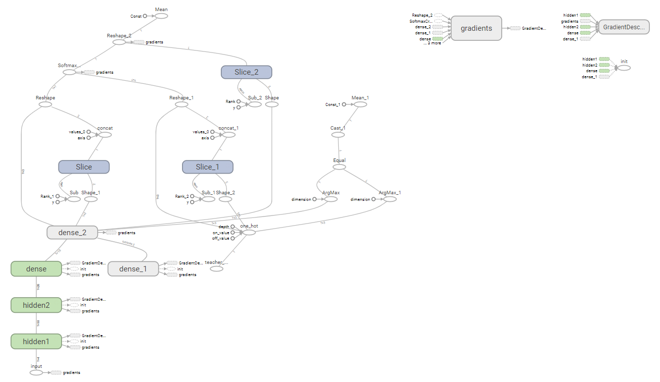
参考に、この計算グラフを以下に示します。

前述のコードで、全てのTensorflow用の変数が「./models/model.ckpt」指定で保存されています。
つまりニューラルネットワークの深層学習で得られた、重みやバイアスの内部パラメタが変数なので、 それを復元「saver.restore」して、別途にデータを加えて判定する処理に利用できます。
いわゆる「分類器」と呼ばれる処理です。

前述のコードで不要なコードを削除して、
セッションの実行部を、ニューラルネットワークの入力で調べたい パラメタ「[5.9, 3.0, 4.2, 1.5]」を設定して評価するように変更した例です。

# -*- coding: utf-8 -*-
#  <meta charset="utf-8"> iris_3.py
import numpy as np
import tensorflow as tf

# 入力層の入力数が４で、プレイスフォルダを生成
x = tf.placeholder( tf.float32,[ None , 4] , name='input')

# 上記 inputの4入力を持つ10要素の隠れ層を、hidden1の名前で作る。（活性化関数にreluを使う）
hidden1=tf.layers.dense(inputs=x, units=10, activation=tf.nn.relu, name="hidden1")

# 上記 hidden1の10入力を持つ20要素の隠れ層を、hidden2の名前で作る。（活性化関数にreluを使う）
hidden2=tf.layers.dense(inputs=hidden1, units=20, activation=tf.nn.relu, name="hidden2")

# 上記 hidden2の20入力を持つ10要素の隠れ層を作る。（活性化関数にreluを使う）
hidden3=tf.layers.dense(inputs=hidden2, units=10, activation=tf.nn.relu)

# 上記 hidden3の10入力を持つ3要素の出力層を作る。（活性化関数にsoftmaxを使う）
y=tf.layers.dense(inputs=hidden3, units=3, activation=tf.nn.softmax)


checkpoint_state = tf.train.get_checkpoint_state("./models/") # 保存したチェックポイント情報取得
print("保存情報:", checkpoint_state.model_checkpoint_path)
saver = tf.train.Saver() # 読み込みの準備

with tf.Session() as sess: # 学習、テスト評価をスタート
   sess.run( tf.global_variables_initializer() )
   saver.restore(sess, "./models/model.ckpt") # これでファイル群から保存時の変数に復元している。 
   result = sess.run( y , feed_dict={ x: np.array([[5.9, 3.0,  4.2, 1.5]]) } )
   idxmax = result[0].argmax() # 最も大きな要素の添え字を取得
   print(result, "：品種判定結果：", idxmax)

以上をiris_3.pyで作成し、その実行結果例は、次のようになります。

my2) F:\python_ai\tensortest>python iris_3.py
保存情報: ./models/model.ckpt
[[5.7963804e-05 9.9912459e-01 8.1738672e-04]] ：品種判定結果： 1

(my2) F:\python_ai\tensortest>

[1]の要素の「 9.9912459e-01 」の確率値が最も大きいという結果を意味します。
[]の中が各品種と判定する予想の確率なので、「5.7963804e-05 + 9.9912459e-01 + 8.1738672e-04」
の値は１になります。（実際は、１に近いの0.999999940524値ですが・・）
さて、実はxへの入力パラメタは、検証のためテスト用のデータを使いました。
全てのテストデータを、順番に検証するプログラムに変更してみます。
その場合、上記の「with tf.Session() as sess: # 学習、テスト評価をスタート」以降を次のように変更することでできます。

IRIS_TEST = 'iris_test.csv' # テスト用
test_data = np.loadtxt('./' + IRIS_TEST, delimiter=",", skiprows=1)
test_x = test_data[:, :-1] # 先頭列から、後方より1列までを抽出
test_y = test_data[:, -1] # 最終列だけを一次元で抽出
print("test_x.shape, test_y.shape:",test_x.shape, test_y.shape) # test_x.shape, test_y.shape:(30, 4) (30,)
print("以下がテストデータ")
print(test_x)
print("以上\n以下がテストデータの正解ラベル")
print(test_y)
print("----データの読み込み終了---------", )

with tf.Session() as sess: # 学習、テスト評価をスタート
   sess.run( tf.global_variables_initializer() )
   saver.restore(sess, "./models/model.ckpt") # これでファイル群から保存時の変数に復元している。 
   for i in range(test_x.shape[0]):
      print( [ test_x[i] ], "入力の結果=>", end="" )
      result = sess.run( y , feed_dict={ x: [ test_x[i] ] } )
      idxmax = result[0].argmax() # 最も大きな要素の添え字を取得
      print(result, "：品種判定結果：", idxmax)

この実行例を以下に示します。

(my2) F:\python_ai\tensortest>python iris_3.py
保存情報: ./models/model.ckpt
test_x.shape, test_y.shape: (30, 4) (30,)
以下がテストデータ
[[5.9 3.  4.2 1.5]
 [6.9 3.1 5.4 2.1]
 [5.1 3.3 1.7 0.5]
 [6.  3.4 4.5 1.6]
 [5.5 2.5 4.  1.3]
 [6.2 2.9 4.3 1.3]
 [5.5 4.2 1.4 0.2]
 [6.3 2.8 5.1 1.5]
 [5.6 3.  4.1 1.3]
 [6.7 2.5 5.8 1.8]
 [7.1 3.  5.9 2.1]
 [4.3 3.  1.1 0.1]
 [5.6 2.8 4.9 2. ]
 [5.5 2.3 4.  1.3]
 [6.  2.2 4.  1. ]
 [5.1 3.5 1.4 0.2]
 [5.7 2.6 3.5 1. ]
 [4.8 3.4 1.9 0.2]
 [5.1 3.4 1.5 0.2]
 [5.7 2.5 5.  2. ]
 [5.4 3.4 1.7 0.2]
 [5.6 3.  4.5 1.5]
 [6.3 2.9 5.6 1.8]
 [6.3 2.5 4.9 1.5]
 [5.8 2.7 3.9 1.2]
 [6.1 3.  4.6 1.4]
 [5.2 4.1 1.5 0.1]
 [6.7 3.1 4.7 1.5]
 [6.7 3.3 5.7 2.5]
 [6.4 2.9 4.3 1.3]]
以上
以下がテストデータの正解ラベル
[1. 2. 0. 1. 1. 1. 0. 2. 1. 2. 2. 0. 2. 1. 1. 0. 1. 0. 0. 2. 0. 1. 2. 1.
 1. 1. 0. 1. 2. 1.]
----データの読み込み終了---------
[array([5.9, 3. , 4.2, 1.5])] 入力の結果=>[[5.7963804e-05 9.9912459e-01 8.1738672e-04]] ：品種判定結果： 1
[array([6.9, 3.1, 5.4, 2.1])] 入力の結果=>[[1.4234229e-10 5.5139493e-03 9.9448603e-01]] ：品種判定結果： 2
[array([5.1, 3.3, 1.7, 0.5])] 入力の結果=>[[9.9869305e-01 1.3069884e-03 2.8836678e-16]] ：品種判定結果： 0
[array([6. , 3.4, 4.5, 1.6])] 入力の結果=>[[2.0710655e-05 9.9703491e-01 2.9444047e-03]] ：品種判定結果： 1
[array([5.5, 2.5, 4. , 1.3])] 入力の結果=>[[5.7612571e-05 9.9485910e-01 5.0832373e-03]] ：品種判定結果： 1
[array([6.2, 2.9, 4.3, 1.3])] 入力の結果=>[[1.1257207e-04 9.9983895e-01 4.8536982e-05]] ：品種判定結果： 1
[array([5.5, 4.2, 1.4, 0.2])] 入力の結果=>[[9.9968815e-01 3.1183238e-04 8.7043337e-19]] ：品種判定結果： 0
[array([6.3, 2.8, 5.1, 1.5])] 入力の結果=>[[5.3368186e-08 1.6162336e-01 8.3837658e-01]] ：品種判定結果： 2
[array([5.6, 3. , 4.1, 1.3])] 入力の結果=>[[1.4345240e-04 9.9956435e-01 2.9214041e-04]] ：品種判定結果： 1
[array([6.7, 2.5, 5.8, 1.8])] 入力の結果=>[[5.7470081e-14 2.7851283e-05 9.9997211e-01]] ：品種判定結果： 2
[array([7.1, 3. , 5.9, 2.1])] 入力の結果=>[[6.5759152e-14 4.3843022e-05 9.9995613e-01]] ：品種判定結果： 2
[array([4.3, 3. , 1.1, 0.1])] 入力の結果=>[[9.9815720e-01 1.8428154e-03 8.6004566e-15]] ：品種判定結果： 0
[array([5.6, 2.8, 4.9, 2. ])] 入力の結果=>[[4.6915397e-12 1.1052409e-04 9.9988949e-01]] ：品種判定結果： 2
[array([5.5, 2.3, 4. , 1.3])] 入力の結果=>[[3.3669163e-05 9.8160708e-01 1.8359229e-02]] ：品種判定結果： 1
[array([6. , 2.2, 4. , 1. ])] 入力の結果=>[[2.9134887e-04 9.9968648e-01 2.2109562e-05]] ：品種判定結果： 1
[array([5.1, 3.5, 1.4, 0.2])] 入力の結果=>[[9.9930656e-01 6.9349183e-04 5.0212623e-17]] ：品種判定結果： 0
[array([5.7, 2.6, 3.5, 1. ])] 入力の結果=>[[9.1266828e-03 9.9087310e-01 2.2082327e-07]] ：品種判定結果： 1
[array([4.8, 3.4, 1.9, 0.2])] 入力の結果=>[[9.9876773e-01 1.2322941e-03 3.3607509e-16]] ：品種判定結果： 0
[array([5.1, 3.4, 1.5, 0.2])] 入力の結果=>[[9.9926192e-01 7.3802716e-04 6.4748926e-17]] ：品種判定結果： 0
[array([5.7, 2.5, 5. , 2. ])] 入力の結果=>[[8.4758052e-13 4.1940766e-05 9.9995804e-01]] ：品種判定結果： 2
[array([5.4, 3.4, 1.7, 0.2])] 入力の結果=>[[9.9937719e-01 6.2281912e-04 1.7512588e-17]] ：品種判定結果： 0
[array([5.6, 3. , 4.5, 1.5])] 入力の結果=>[[3.8375756e-06 7.5873476e-01 2.4126145e-01]] ：品種判定結果： 1
[array([6.3, 2.9, 5.6, 1.8])] 入力の結果=>[[4.4041290e-13 6.7323672e-05 9.9993265e-01]] ：品種判定結果： 2
[array([6.3, 2.5, 4.9, 1.5])] 入力の結果=>[[1.1543994e-07 2.2754674e-01 7.7245313e-01]] ：品種判定結果： 2
[array([5.8, 2.7, 3.9, 1.2])] 入力の結果=>[[5.2555121e-04 9.9946195e-01 1.2462220e-05]] ：品種判定結果： 1
[array([6.1, 3. , 4.6, 1.4])] 入力の結果=>[[1.2103922e-05 9.9391741e-01 6.0705603e-03]] ：品種判定結果： 1
[array([5.2, 4.1, 1.5, 0.1])] 入力の結果=>[[9.9959785e-01 4.0214907e-04 3.3668912e-18]] ：品種判定結果： 0
[array([6.7, 3.1, 4.7, 1.5])] 入力の結果=>[[1.8732948e-05 9.9972028e-01 2.6105225e-04]] ：品種判定結果： 1
[array([6.7, 3.3, 5.7, 2.5])] 入力の結果=>[[2.1112794e-14 1.3185021e-05 9.9998677e-01]] ：品種判定結果： 2
[array([6.4, 2.9, 4.3, 1.3])] 入力の結果=>[[1.6986378e-04 9.9982041e-01 9.7524708e-06]] ：品種判定結果： 1

(my2) F:\python_ai\tensortest>